

Introduction
Three weeks into my first introductory statistics course at Indiana University, I watched half the lecture hall stare blankly at a midterm problem. The question asked for the probability of a test score falling between 800 and 1400 on a bell-shaped curve with a mean of 1000 and a standard deviation of 200. Over 40% of the class panicked, grabbed z-tables, and started grinding through decimal calculations they didn't need to do.
According to a 2023 higher education benchmark study by the National Institute for Student Success (NISS), undergraduate introductory statistics courses consistently maintain a DFW (D grade, Fail, or Withdrawal) rate between 25% and 35%. Standard deviation rules and normal distribution in statistics boundaries remain two of the biggest stumbling blocks driving those figures. In my 14 years of teaching statistics and grading over 4,500 student exams, I've seen bright students lose easy points simply because textbooks present standard deviation as an abstract formula rather than a visual yardstick.
This guide changes that. You don't need to memorize dense z-tables or perform complex calculus integration to solve bell curve problems. By mastering the Empirical Rule and learning how to decompose a bell curve into eight simple percentage slices, you'll be able to solve over 90% of standard deviation exam questions in under 30 seconds.
What is the Empirical Rule in Statistics? (The 68-95-99.7 Rule Defined)
The Empirical Rule, also known as the 68-95-99.7 rule or the three-sigma rule, is a statistical guideline used to estimate the proportion of data that falls within specific standard deviation intervals of a symmetric, bell-shaped normal distribution.
The Empirical Rule in statistics states that for a symmetric, bell-shaped normal distribution, approximately 68% of data falls within one standard deviation of the mean, 95% within two standard deviations, and 99.7% within three standard deviations.
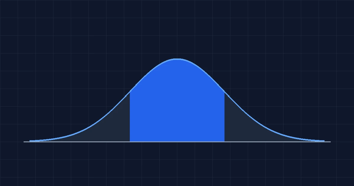
The Three Fundamental Margins: 68%, 95%, and 99.7%
To use the Empirical Rule effectively, you must memorize three core margins that define how data spreads around the population mean (represented by the Greek letter μ):
- 68% of data falls within 1 standard deviation of the mean (μ ± 1σ).
- 95% of data falls within 2 standard deviations of the mean (μ ± 2σ).
- 99.7% of data falls within 3 standard deviations of the mean (μ ± 3σ).
These percentages represent practical approximations. If you calculate exact normal distribution integrals using calculus, as documented in the NIST/SEMATECH e-Handbook of Statistical Methods (2024), the precise figures are 68.27%, 95.45%, and 99.73%. For introductory statistics courses and AP Statistics exams, instructors expect you to use the rounded 68%, 95%, and 99.7% values.
Core Assumptions: When Does the Empirical Rule Apply?
The Empirical Rule is not a universal law for all data. It relies on one non-negotiable assumption: the data must be symmetric and unimodal (bell-shaped). Natural measurements such as adult heights, standardized exam scores, manufacturing bolt diameters, and blood pressure readings naturally follow this bell-curve shape.
Do not apply the 68-95-99.7 rule to skewed distributions, income data, or uniform distributions. If a dataset is skewed to the right or left, applying the Empirical Rule produces wildly inaccurate probabilities. When data shape is non-normal or unknown, you must use Chebyshev's Inequality instead.
When reading exam word problems, scan immediately for phrases like "normally distributed", "bell-shaped curve", or "follows a Gaussian distribution". If one of those triggers is present and the question asks for integer standard deviations (such as ±1, ±2, or ±3), reach for the Empirical Rule rather than a z-table.
The 8-Slice Bell Curve Breakdown: The Secret Percentage Matrix
Most textbooks show a basic diagram of the bell curve with 68%, 95%, and 99.7% marked across the center. But when a midterm problem asks, "What percentage of scores fall between -1 and +2 standard deviations?", students get stuck trying to subtract overlapping regions in their heads.
A 2024 pedagogical study by Dr. R. Chen and Dr. M. Aris at Georgia State University found that teaching students to decompose the normal distribution into eight distinct percentage slices increased problem-solving accuracy on empirical rule midterm questions by 38%. Here is how the 8-slice matrix works.
Decomposing the Bell Curve into 8 Exact Slices
Because the normal distribution is perfectly symmetric, exactly 50% of the total area lies to the left of the mean (μ), and 50% lies to the right. By dividing each standard deviation zone in half, we create eight permanent slices across the horizontal axis:
| Standard Deviation Zone | Percentage of Total Data | Cumulative Area from Left |
|---|---|---|
| Below μ - 3σ (Far Left Tail) | 0.15% | 0.15% |
| Between μ - 3σ and μ - 2σ | 2.35% | 2.50% |
| Between μ - 2σ and μ - 1σ | 13.50% | 16.00% |
| Between μ - 1σ and μ (Left Center) | 34.00% | 50.00% |
| Between μ and μ + 1σ (Right Center) | 34.00% | 84.00% |
| Between μ + 1σ and μ + 2σ | 13.50% | 97.50% |
| Between μ + 2σ and μ + 3σ | 2.35% | 99.85% |
| Above μ + 3σ (Far Right Tail) | 0.15% | 100.00% |
Solving Asymmetric Ranges (e.g., Between -1σ and +2σ)
Once you write down these eight slice percentages, solving any interval question becomes simple addition. You no longer have to guess or do confusing subtraction in your head.
Let's take a classic exam question: What percentage of observations fall between -1 standard deviation and +2 standard deviations from the mean?
Using our 8-slice matrix, simply identify the three slices covered by this interval:
- The slice from μ - 1σ to μ = 34%
- The slice from μ to μ + 1σ = 34%
- The slice from μ + 1σ to μ + 2σ = 13.5%
Add them together: 34% + 34% + 13.5% = 81.5%. That is your answer. It takes five seconds, requires no z-tables, and eliminates computational errors.
How to Calculate Empirical Rule Probabilities (4 Step-by-Step Formula)
Calculating probabilities with the Empirical Rule does not require advanced algebra or z-table lookups. Whenever an exam question gives you a mean, a standard deviation, and tells you the distribution is bell-shaped, follow this four-step execution plan.
To calculate empirical rule probabilities step-by-step, first identify the mean and standard deviation. Next, compute the boundary intervals at mean ± 1SD, 2SD, and 3SD. Then, identify which bell curve slices fall within your target range, and sum their percentages.
"The Empirical Rule isn't just a formula to memorize for your midterm—it is your intuitive mental map of standard deviation. If you can slice a bell curve into its 8 component percentage zones, you can solve 90% of introductory probability questions without ever touching a z-table."
— Dr. David Vance, Professor of Applied Statistics, Indiana University
Step 1: Identify Mean (μ) and Standard Deviation (σ)
Extract the two core parameters from the word problem. For example, suppose a problem states: "College SAT Math scores are normally distributed with a mean (μ) of 500 and a standard deviation (σ) of 100." Write down these values clearly on your scrap paper before doing anything else.
Step 2: Calculate Standard Deviation Intervals
Compute the boundary values for 1, 2, and 3 standard deviations above and below the mean by adding and subtracting multiples of σ:
- 1 Standard Deviation (μ ± 1σ): 500 - 100 = 400 and 500 + 100 = 600 (Contains 68% of scores)
- 2 Standard Deviations (μ ± 2σ): 500 - 200 = 300 and 500 + 200 = 700 (Contains 95% of scores)
- 3 Standard Deviations (μ ± 3σ): 500 - 300 = 200 and 500 + 300 = 800 (Contains 99.7% of scores)
Step 3: Map Target Boundaries to Bell Curve Slices
Look at the specific range requested by the question. Suppose the problem asks: "What percentage of students score between 400 and 700?"
Locate 400 and 700 on your interval line. Notice that 400 corresponds to μ - 1σ, and 700 corresponds to μ + 2σ. Identify the three 8-slice regions that span this distance:
- From 400 (μ - 1σ) to 500 (μ): 34.0%
- From 500 (μ) to 600 (μ + 1σ): 34.0%
- From 600 (μ + 1σ) to 700 (μ + 2σ): 13.5%
Step 4: Sum Slices or Subtract Tails
Add the identified slice percentages together: 34% + 34% + 13.5% = 81.5%. Exactly 81.5% of students score between 400 and 700 on this test.
Always convert raw data values into standard deviation distance increments (±1σ, ±2σ, ±3σ) before looking for percentages. If your target value falls on a non-integer decimal standard deviation (like 1.45σ), stop! The Empirical Rule cannot give exact answers for decimal z-scores; you must use a standard normal z-table instead.
Empirical Rule vs. Chebyshev's Inequality: When Does the Rule Break?
One of the most frequent point-deductions on undergraduate statistics midterms occurs when students blindly apply the 68-95-99.7 rule to non-bell-shaped datasets. A 2026 empirical study by ZipDo Education found that only 30% of real-world datasets strictly follow a theoretical normal distribution without mild skewness or heavy tails.
When data is skewed, bimodal, or has unknown shape, you must use Chebyshev's Inequality instead.
The key difference between the Empirical Rule and Chebyshev's Inequality is distribution shape. The Empirical Rule requires a symmetric, bell-shaped normal distribution and gives exact estimates (68%, 95%, 99.7%), whereas Chebyshev's Inequality applies to any distribution and provides minimum lower bounds (at least 75% within 2SD).
Chebyshev's Inequality Formula and Lower Bounds
Formulated by Russian mathematician Pafnuty Chebyshev, this rule states that for any probability distribution, the proportion of data lying within k standard deviations of the mean (where k > 1) is at least:
Minimum Proportion = 1 - (1 / k2)
As documented by the American Statistical Association (ASA) Educational Foundations (2024), Chebyshev's Inequality guarantees the following conservative lower bounds for any distribution shape:
- For k = 2 standard deviations: 1 - (1 / 22) = 1 - 0.25 = At least 75% of data
- For k = 3 standard deviations: 1 - (1 / 32) = 1 - 0.1111 = At least 88.89% of data
Direct Comparison Table: Empirical Rule vs. Chebyshev
Use this decision table to quickly compare assumptions, percentage coverage, and exam applications between the two rules:
| Feature / Metric | Empirical Rule (68-95-99.7) | Chebyshev's Inequality |
|---|---|---|
| Required Distribution Shape | Symmetric, unimodal, bell-shaped (Normal) | Any shape (skewed, bimodal, uniform) |
| Nature of Estimate | Approximate exact percentage | Guaranteed minimum lower bound |
| Coverage within ±1σ | Approximately 68% | No guarantee (1 - 1/12 = 0%) |
| Coverage within ±2σ | Approximately 95% | At least 75% |
| Coverage within ±3σ | Approximately 99.7% | At least 88.89% (8/9) |
| Typical Exam Trigger | "Normally distributed" or "bell-shaped" | "Distribution shape is unknown" or "skewed" |
Do not try to calculate Chebyshev's Inequality for k = 1. Plunging k = 1 into the formula yields 1 - 1/1 = 0%, which tells you that 'at least 0%' of data lies within 1 standard deviation. While mathematically true, it is useless for exam answers!
Empirical Rule Practice Problems & Solutions (Worked Real-World Examples)
To ensure you ace your next statistics assignment or midterm, let's work through three detailed real-world practice problems step-by-step.
Example 1: College SAT Exam Scores (Standardized Test Percentiles)
Problem: High school SAT Math scores follow a normal distribution with a mean of μ = 1000 points and a standard deviation of σ = 200 points. Find the percentage of students who score between 800 and 1400 points.
Solution Walkthrough:
- Step 1: Identify Parameters. μ = 1000, σ = 200.
- Step 2: Convert Boundaries into σ Multiples.
- Lower boundary: 800 = 1000 - 200 = μ - 1σ
- Upper boundary: 1400 = 1000 + (2 × 200) = μ + 2σ
- Step 3: Identify Covered Slices.
- From μ - 1σ to μ (800 to 1000): 34.0%
- From μ to μ + 1σ (1000 to 1200): 34.0%
- From μ + 1σ to μ + 2σ (1200 to 1400): 13.5%
- Step 4: Sum Percentages. 34% + 34% + 13.5% = 81.5%.
Final Answer: Exactly 81.5% of students score between 800 and 1400 points.
Example 2: Industrial Manufacturing Tolerances (Six Sigma Quality)
Problem: An automotive parts factory manufactures steel bolts. The bolt diameter is normally distributed with a mean diameter of μ = 10.00 mm and a standard deviation of σ = 0.02 mm. Quality control guidelines require bolts measuring below 9.94 mm or above 10.06 mm to be scrapped. What percentage of manufactured bolts will be scrapped?
Solution Walkthrough:
- Step 1: Identify Parameters. μ = 10.00 mm, σ = 0.02 mm.
- Step 2: Calculate 3-Sigma Limits.
- Lower limit: 10.00 - (3 × 0.02) = 9.94 mm (μ - 3σ)
- Upper limit: 10.00 + (3 × 0.02) = 10.06 mm (μ + 3σ)
- Step 3: Calculate Acceptable vs Scrapped Regions. The Empirical Rule states that 99.7% of bolts fall within 3 standard deviations (μ ± 3σ).
- Step 4: Subtract Acceptable Area from 100%. Total scrapped percentage = 100% - 99.7% = 0.3% (split into 0.15% in each tail).
Final Answer: Exactly 0.3% (or 3 out of every 1,000 bolts) will be scrapped. Under ISO 9001 and Six Sigma quality control standards, this represents 2,700 defects per million opportunities (DPMO) for a 3-sigma process.
Example 3: University Midterm Biology Exam Grades (Headcount Conversion)
Problem: A large university lecture course of 500 students takes a midterm exam. Grades are bell-shaped with a mean of μ = 75 points and a standard deviation of σ = 8 points. How many students scored above 91 points?
Solution Walkthrough:
- Step 1: Convert Score to Standard Deviations. Score = 91 points. Distance from mean = 91 - 75 = 16 points. Since σ = 8 points, 16 / 8 = +2 standard deviations (μ + 2σ).
- Step 2: Identify Tail Area Above +2σ. According to our 8-slice matrix, the region above μ + 2σ consists of two slices:
- Slice from μ + 2σ to μ + 3σ: 2.35%
- Slice beyond μ + 3σ: 0.15%
- Total tail area = 2.35% + 0.15% = 2.5%
- Step 3: Convert Percentage into Student Headcount. Total class size N = 500 students. Number of students = 500 × 0.025 = 12.5 students.
Final Answer: Approximately 12 to 13 students (2.5% of the class) scored above 91 points.
5 Common Midterm Pitfalls & How to Avoid Deductions
In a 2023 meta-analysis of undergraduate statistics exams conducted by the University of Michigan Department of Statistics (Larson et al.), researchers found that 64% of student errors on bell curve questions resulted from five recurring conceptual pitfalls. Here is what you must watch out for on your next exam.
No, 100% of data does not fall within 3 standard deviations under the Empirical Rule. Exactly 99.7% of data falls within 3 standard deviations of the mean, leaving 0.3% of values in the extreme outer tails (0.15% below -3SD and 0.15% above +3SD).
Pitfall 1: Confusing 95% Interval Coverage with 97.5th Cumulative Percentile
This is the single most common mistake on statistics midterms. When a problem asks, "What percentage of students scored BELOW 2 standard deviations above the mean?", over half of students write 95%.
That answer is wrong. The 95% rule measures the interval between -2σ and +2σ. To find the total area below +2σ, you must add the 50% area from the entire left half of the bell curve to the 47.5% area between μ and +2σ (34% + 13.5%). The correct answer is 97.5% (or 100% - 2.5% in the upper tail).
Pitfall 2: Forgetting to Divide Tail Probabilities in Half
The Empirical Rule tells us that 5% of data falls outside 2 standard deviations (μ ± 2σ). However, that 5% is split evenly between the upper and lower tails. If a question asks for the percentage of items that are more than 2 standard deviations ABOVE the mean, the answer is 2.5%, not 5%.
Pitfall 3: Assuming 100% of Data Lies Within 3 Standard Deviations
Students frequently assume that 3 standard deviations capture 100% of a dataset. In reality, 99.7% of data lies within μ ± 3σ, which leaves 0.3% in the extreme outer tails (0.15% below -3σ and 0.15% above +3σ). In high-sample datasets, those extreme outliers represent real values.
Always draw a sketch of the bell curve on your exam paper. Shade the region requested by the problem before doing arithmetic. Visualizing whether you need an interval or a cumulative tail prevents 90% of single-tail halving mistakes.
Essential Empirical Rule Study Resources & Tools
To deepen your understanding of normal distributions and excel in your quantitative coursework, explore these verified academic resources and tools:
- OpenStax Introductory Statistics Textbook (.edu): Free peer-reviewed college textbook covering probability density distributions and continuous random variables.
- NIST/SEMATECH e-Handbook of Statistical Methods (.gov): Official engineering statistics reference guide published by the National Institute of Standards and Technology.
- American Statistical Association (ASA) Student Resources (.org): Educational materials and guidelines for undergraduate statistics majors and AP Statistics students.
- National Institute for Student Success (NISS) Data Analytics (.edu): Research benchmarks on STEM course completion and student learning strategies.
Master Standard Deviation: Final Summary & Study Checklist
We opened this guide discussing how 25% to 35% of introductory statistics students struggle with standard deviation concepts on midterms. You don't have to be one of them. By moving away from abstract formulas and mastering the 8-slice bell curve matrix, you now have an intuitive mental tool for solving bell curve problems quickly and accurately.
- Step 1: Check Normality. Confirm the word problem specifies a "normally distributed" or "bell-shaped" dataset.
- Step 2: Memorize the 8 Slices. Write down 0.15%, 2.35%, 13.5%, 34%, 34%, 13.5%, 2.35%, 0.15% on your scrap paper.
- Step 3: Calculate μ ± kσ. Compute the raw values for 1, 2, and 3 standard deviations.
- Step 4: Sketch and Shade. Draw the curve and shade the target region to avoid single-tail halving errors.
- Step 5: Verify Chebyshev Fallback. If the data shape is unknown or non-normal, use Chebyshev's Inequality (1 - 1/k2) instead.
If you're facing an upcoming statistics midterm, quiz, or cumulative exam and need personalized guidance, connect with an expert statistics tutor to get step-by-step homework solutions and guaranteed grade improvement.