
Two weeks into my first college biostatistics course, I made a mistake that still makes me cringe. I was calculating the median of a list of ten patient weights, got the math completely right, but received a zero on the exam question. Why? I forgot to sort the dataset in ascending order before finding the middle value. I knew the definition by heart, but in the rush of the exam, the basic procedure fell apart. That is the median error, and it is one of the most common ways students lose points they thought they had secured.
This is the classic descriptive statistics trap. Calculating the mean, median, and mode is middle school arithmetic. But knowing which one to use, and how to interpret them without misleading your audience, is college statistics. In my office hours, I see dozens of students every semester who can calculate a decimal average in their sleep, but freeze when an exam question asks them to justify their choice of central tendency for a skewed real estate dataset.
The numbers back this up. In a 2006 study published in Educational Studies in Mathematics, researchers Randall Groth and Jennifer Bergner analyzed pre-service teachers and found that only 7% could successfully discuss the conceptual suitability of different measures of central tendency for real-world contexts. Additionally, a 2019 review by the International Association for Statistical Education (IASE) revealed that 85% of homework exercises in introductory textbooks focus purely on calculation. Fewer than 15% ask students to select or justify their choice of measure. Standard courses train you to compute, not to reason.
This guide changes that. We will skip the dry textbook formulas and focus on the practical decision rules you need for homework and exams. You will learn the physics behind the mean, the physical lineup that defines the median, and the reason the mode is your only option for qualitative categories. We will also expose the three classic exam traps professors use to catch students off guard. These strategies are drawn from my 12 years of teaching and grading college statistics exams.
What Is Central Tendency? The Three Pillars of Data Summary
A measure of central tendency is a single representative value that attempts to describe a set of data by identifying the central position within that dataset. In introductory statistics, the three primary measures used to identify this center are the mean, the median, and the mode. They each define the middle in a fundamentally different way, which is why they often produce different numbers for the exact same dataset.
The term central tendency refers to the tendency of quantitative data to cluster around some central value. When you are handed a raw spreadsheet containing 10,000 patient blood pressure readings, your brain cannot process the raw numbers. You need a summary. You need a single value that tells you what a typical reading looks like. That is what these three measures provide, but each measure highlights a different property of the distribution.
The Three Definitions
The arithmetic mean is the mathematical center, calculated by summing all observations and dividing by the total count. The median is the physical midpoint, dividing the sorted dataset into two equal halves. The mode is the peak frequency, representing the value that appears most often. Most textbooks stop here, but the real difficulty lies in understanding that these are not interchangeable tools.
In their Guidelines for Assessment and Instruction in Statistics Education (GAISE) Report, the American Statistical Association (ASA) emphasizes that sound statistical reasoning requires examining the data distribution before choosing a summary statistic. No single measure of center is best for every situation. Choosing the wrong measure does not just lead to a bad grade, it actively misleads whoever reads your research.
A Simple Example
Let us look at a real dataset to see how these three pillars differ. Suppose you track the number of daily study hours for five students: {2, 3, 3, 4, 8}.
- To find the mean, you add all values to get 20, then divide by 5. The mean is 4 hours.
- To find the median, you sort the values and find the middle number. The median is 3 hours.
- To find the mode, you locate the most frequent number. The mode is 3 hours.
While the mean (4) is pulled upward by the student studying 8 hours, the median and mode remain at 3. Each number is correct, but they tell different stories about the typical student's behavior.
The Origins of Center: How Mean, Median, and Mode Came to Be
The measures of central tendency did not emerge as a unified statistical toolkit. They were invented centuries apart by scholars trying to solve completely unrelated problems. Knowing where these tools came from helps explain why they behave so differently on your exams.
The concept of the arithmetic average, or mean, is the oldest of the three. Its roots go back to ancient Greece, where Pythagoras and his followers defined three mathematical means: the arithmetic, the geometric, and the harmonic. In the ancient world, these means were used to analyze musical scales and geometric proportions, not observational data. It was not until 1632 that the Italian astronomer Galileo Galilei, in his work Dialogue Concerning the Two Chief World Systems, suggested using the arithmetic mean to estimate the true position of a star by averaging conflicting astronomical observations. Galileo realized that random measurement errors tended to cancel each other out when summed and divided.
The median arrived much later as a navigation hack. In 1599, the English mathematician Edward Wright published Certaine Errors in Navigation, where he proposed using the middle value of a set of compass measurements rather than the mean. Wright knew that if a navigator made nine sightings, the middle observation would minimize the risk of a single wild error throwing off the entire ship's course. In 1843, the French economist Antoine Augustin Cournot formally defined the median in a mathematical context, introducing it as the value where the probability of exceeding it is equal to the probability of falling short.
The mode is the youngest of the three terms. The English statistician Karl Pearson coined the term in his 1895 paper, Contributions to the Mathematical Theory of Evolution. Pearson, who was studying skewed biological distributions, needed a term for the peak of a curve, the value of maximum frequency. He chose the word mode, which is derived from the French phrase à la mode, meaning fashionable or popular. Pearson's linguistic choice was literal: the mode is simply the most popular value in the dataset.
This history shows that the mean was built for physical science measurements where errors are symmetric, whereas the median was built to resist extreme, navigational errors. Today, these historical differences shape real-world reporting. For example, the U.S. Census Bureau reported that the real median household income in 2023 was $80,610, while the mean household income was significantly higher at $135,700 for families. The high-income outliers pull the mean upward, just as a wild measurement error would have done to Edward Wright's navigation calculations in 1599. When you choose between the mean and median on an exam, you are choosing between Galileo's error-averaging logic and Wright's outlier-resistant midpoint.
When to Use the Mean: The See-Saw Balance Point
The arithmetic mean is the most popular measure of central tendency, but it is also the most misunderstood. Mathematically, you calculate it by adding every single value in your dataset and dividing by the total number of observations. Conceptually, however, the mean is not just an average. It is a physical balance point, much like the fulcrum of a see-saw.
Imagine a long wooden plank with weights placed at different positions along its length. If you want the plank to sit perfectly level without tipping, you must place the support fulcrum at the exact center of gravity. That center of gravity is the arithmetic mean. If you shift a single weight even a fraction of an inch to the right, the entire balance point shifts to the right to compensate. This physical sensitivity is both the mean's greatest strength and its primary weakness.
Because the mean uses every single data point in its calculation, it is highly representative when your data is distributed symmetrically. For example, let us look at a set of quiz scores from five students in my introductory class: {80, 82, 85, 88, 90}. The sum of these scores is 425. When we divide by 5, we get a mean score of 85. This number represents the center of gravity for the quiz performance. It is a highly informative metric because it reflects the performance of every student in the group.
However, this sensitivity makes the mean highly vulnerable to distortion. If one student fails the quiz with a score of 10, the dataset becomes {10, 82, 85, 88, 90}. The sum drops to 355, and the new mean falls to 71. Suddenly, the balance point has shifted dramatically downward, even though four out of the five students still scored an 82 or higher. The mean of 71 tells a misleading story about the class's typical performance because it has been dragged down by a single low score.
For this reason, you should only use the mean when your data is continuous (interval or ratio level of measurement) and follows a symmetric, bell-shaped distribution. If your data contains extreme values, the mean will give you a distorted view of the center.
Many students make the mistake of using the mean for qualitative ordinal data, such as satisfaction surveys. A 2004 study by Susan Jamieson, published in the journal Medical Education and hosted on the National Institutes of Health website (nih.gov), warns that treating ordinal Likert scale responses (such as 1 for Strongly Disagree and 5 for Strongly Agree) as interval data to calculate a mean is a major methodological error. You cannot average categories because the distance between the numbers is not mathematically equal. The mean of ordinal data is statistically meaningless.
When to Use the Median: The Physical Midpoint
If the mean is a see-saw balance point, the median is a physical lineup. The median is the exact 50th percentile of your dataset. It is the value that splits an ordered dataset into two equal halves, ensuring that 50% of the observations fall below it and 50% fall above it.
To understand the median, imagine lining up all the students in a classroom from shortest to tallest. The median is the height of the person standing at the exact middle of the line. If there are 21 students in the line, the median is the height of the 11th person. It does not matter if the tallest person in the line is 6 feet tall or 60 feet tall. The physical position of the middle person does not change. This resistance to extreme values is why statisticians call the median a robust measure of central tendency.
There is one mandatory step that students forget on exams: you must sort the dataset in ascending order before locating the median. Calculating the median without sorting is the most common execution error in introductory courses. A 2014 report on mathematics education from the University of Arizona (arizona.edu) noted that students frequently make procedural errors when identifying the median because they treat the raw list as if it represents the spatial distribution of the data.
The rules for calculating the median depend on whether you have an odd or even number of observations.
The Odd Number Rule
If your dataset has an odd number of values, the median is the single value in the exact middle. For example, consider the sorted dataset of daily study hours for five students: {2, 3, 3, 4, 8}. The number of observations is odd, so the median is the third value, which is 3.
The Even Number Rule
If your dataset has an even number of values, there is no single middle number. Instead, you must find the two middle numbers, add them together, and divide by 2. Let us look at a sorted dataset of six test scores: {12, 14, 15, 18, 20, 22}. The two middle values are 15 and 18. To find the median, we add them together to get 33, then divide by 2. The median is 16.5.
The median is the ideal measure of center when your dataset contains extreme outliers or is highly skewed. Because it only cares about the rank order of the numbers, it ignores the actual magnitude of extreme values. A student studying 80 hours a week instead of 8 hours would pull the mean upward, but the median would remain locked at the center of the physical lineup.
When to Use the Mode: The Category Champion
The mode is the simplest measure of central tendency to define: it is the value that occurs most frequently in your dataset. While the mean balances weights and the median finds the middle of a lineup, the mode wins a popularity contest.
The mode is the only measure of central tendency that works for qualitative, nominal data. When you collect data on eye color, favorite brands, or college majors, you cannot add the categories together to calculate a mean, and you cannot sort them to find a median. The only center you can report is the category that appears most often. For example, if you survey 100 students about their favorite major and 45 say Business, 30 say Psychology, and 25 say Biology, the mode is Business. It represents the peak frequency of your categories.
Unlike the mean and median, which always yield a single center, a dataset can have more than one mode. If two values share the highest frequency, the dataset is bimodal. If three or more values share the highest frequency, it is multimodal. If every value appears exactly once, the dataset has no mode at all.
The concept of multiple modes is highly useful in real-world operations. A hospitality management report from Cornell University (cornell.edu) highlights this using restaurant customer arrival times. If a restaurant experiences a lunch rush peak at 12 PM with 50 transactions and a dinner rush peak at 6 PM with 52 transactions, the dataset is bimodal. The peaks occur at 12 PM and 6 PM. If you average these times to find a mean arrival time, you get 3 PM. But 3 PM is the deadest hour of the day, when the kitchen is nearly empty. Using the mean to schedule staff would result in a scheduling disaster. The mode is the only metric that reveals the true peaks in the distribution.
The Distribution Battle: Mean vs. Median vs. Mode in Skewed Data
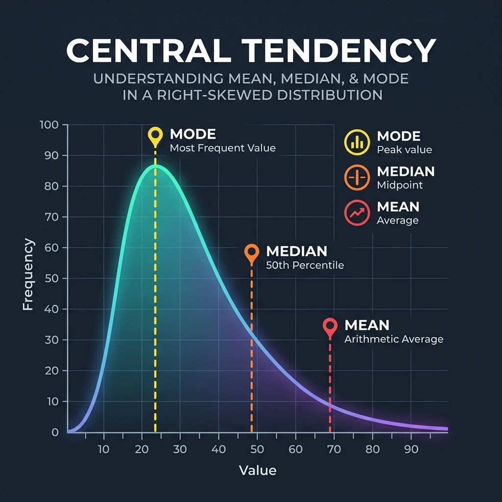
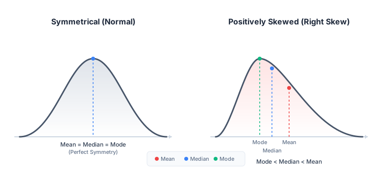
The shape of your data's distribution determines how the mean, median, and mode behave relative to one another. When your distribution is perfectly symmetrical, all three measures point to the exact same value. But when your data is skewed, these measures pull apart in a predictable mathematical tug-of-war.
Symmetrical Distributions
In a normal, bell-shaped distribution, the data is balanced on both sides of the center. The highest peak is in the exact middle, which means the mode is in the center. Because the data is symmetric, the physical midpoint (median) and the mathematical balance point (mean) also align at this exact peak. In this ideal scenario, Mean = Median = Mode.
Positively Skewed (Right-Skewed) Distributions
In a positively skewed distribution, the tail of the curve points to the right. This shape indicates that the majority of the observations are clustered at the lower end of the scale, while a few extreme high values stretch out to the right. These high-value outliers act like heavy weights on a see-saw, dragging the mean toward the right tail. The median, being robust, shifts only slightly, while the mode remains at the highest peak on the left. In a positively skewed distribution, the relationship is always: Mean > Median > Mode.
Real-world income reporting is the classic example of right skewness. According to the U.S. Census Bureau data from 2023, the real median household income in the United States was $80,610, while the mean family income was significantly higher at $135,700. A small percentage of extremely high-income households pulls the mean upward, making it unrepresentative of the typical American household. The median of $80,610 provides a much more realistic picture of the middle class.
Negatively Skewed (Left-Skewed) Distributions
In a negatively skewed distribution, the tail points to the left. This shape occurs when most values are high, but a few extreme low values pull the distribution to the left. These low-value outliers drag the mean downward, while the median remains closer to the bulk of the data, and the mode stays at the highest peak on the right. In a negatively skewed distribution, the relationship is: Mean < Median < Mode.
The Outlier Stress Test
Let us conduct a mathematical experiment to see this tug-of-war in action. We will start with a baseline dataset representing the weekly study hours of five students: {10, 12, 14, 15, 16}.
- Baseline Mean: (10 + 12 + 14 + 15 + 16) / 5 = 13.4 hours.
- Baseline Median: The sorted middle value is 14 hours.
- Baseline Mode: No mode, as all values appear once.
Now, let us introduce a massive outlier to the dataset. Suppose a sixth student enters the group who studies 1,000 hours a week (perhaps a data logging error, but an outlier nonetheless). Our new dataset is: {10, 12, 14, 15, 16, 1000}.
- New Mean: (10 + 12 + 14 + 15 + 16 + 1000) / 6 = 177.83 hours.
- New Median: The two middle values are 14 and 15, so (14 + 15) / 2 = 14.5 hours.
- New Mode: Still no mode.
Look at the percentage change. The mean increased from 13.4 to 177.83, a massive change of 1,227%. A mean of 177 hours suggests the typical student studies over 25 hours a day, which is physically impossible. In contrast, the median only shifted from 14 to 14.5, a minor increase of 3.57%. This calculation proves why the median is the only reliable choice when your data is skewed by outliers.
The Homework Translation Matrix: How to Choose on Exams
When you are in the middle of a statistics exam, you do not have time to second-guess yourself. You need a fast, reliable framework to decide which measure of central tendency is required for a given problem. A study published in the AIP Conference Proceedings in 2020 revealed that nearly 40% of introductory statistics students solve problems involving central tendency measures improperly or fail to show logical work. They memorize the formulas but cannot translate the word problems.
To prevent this, use the lookup matrix below to match your variable type and distribution shape to the optimal measure of center.
| Level of Measurement | Distribution Shape | Optimal Measure | Real-World Example |
|---|---|---|---|
| Nominal (Categories, no order) | Any shape | Mode | Favorite soda brand, eye color, zip codes |
| Ordinal (Ordered categories) | Any shape | Median | Customer satisfaction rating (1 to 5), class rank |
| Interval/Ratio (Continuous, symmetric) | Symmetric (No outliers) | Mean | Standardized test scores, room temperature |
| Interval/Ratio (Continuous, skewed) | Skewed (Outliers present) | Median | Home prices in a city, professional athlete salaries |
Before writing down your answer on an exam, ask yourself two questions. First, what level of measurement is this data? If it is nominal, your search is over: the answer is the mode. Second, if the data is numerical, are there outliers or skewness? If the problem describes home values in Beverly Hills or salaries at a tech startup, you are dealing with a right-skewed distribution. Choose the median.
The 3 Classic Exam Traps Professors Use
Professors know that students rely on rote memory rather than conceptual understanding. To test your true comprehension, we design specific questions that expose common calculation habits. The 2000 study by Watson and Moritz on statistical understanding highlights that between 55% and 74% of school-age students hold key conceptual errors when attempting to describe or calculate the median and mean. These errors persist into college. Here are the three classic traps you will encounter on your exams.
Trap 1: The Unsorted Median List
A professor gives you a raw list of numbers: {8, 2, 15, 6, 12} and asks you to find the median. If you are rushing, you might look at the raw list, count two numbers from the left, two from the right, and identify 15 as the middle value. This is a trap.
To avoid this, you must sort the list in ascending order first: {2, 6, 8, 12, 15}. Now, the middle number is clearly 8. Always write out the sorted list on your scratch paper before identifying the midpoint. This simple habit will save you from losing easy points.
Trap 2: The Bimodal Category Average
An exam question presents a dataset of shirt colors worn by employees: {Red, Red, Blue, Green, Green}. The question asks you to calculate the average shirt color. Many students freeze, wondering how to add colors together and divide by 5.
The trap is the word average. In common language, average refers to the mean. But in statistics, average can refer to any measure of center. Because shirt color is nominal data, you cannot calculate a mean or median. The only valid average is the mode. Since Red and Green both appear twice, the dataset is bimodal. Your answer should state that the average is bimodal, with modes of Red and Green. You cannot calculate a single numerical average for categories.
Trap 3: The Continuous Decimal Mode
You are given a list of high-precision continuous measurements, such as the exact weights of three chemicals in a lab: {150.24, 152.41, 151.87}. The question asks for the mode.
Because no two numbers are identical, many students make the mistake of writing Mode = 0. This is incorrect. Writing Mode = 0 means that the number zero appears most frequently in your dataset. The correct answer is that there is no mode. In continuous datasets with high-precision decimals, it is common to have no mode because measurements rarely repeat exactly.
How to Calculate Measures of Center in Excel, Google Sheets, SPSS, and R
In college statistics courses, you will rarely calculate measures of center by hand once you move past the first exam. In the real world, researchers rely on statistical software. However, each tool has its own quirks and formula names. If you do not know the exact commands, you will waste hours debugging your analysis.
Excel and Google Sheets
Spreadsheet software is the most common tool for basic data
summaries. In both Excel and Google Sheets, you must enter a
specific formula into a cell followed by the range of your
data (for example, A1:A50).
-
Mean: Use the formula
=AVERAGE(range). Excel does not have a formula named=MEAN(), which is a frequent source of confusion for beginners. -
Median: Use the formula
=MEDIAN(range). Remember that Excel sorts the data behind the scenes, so you do not need to sort the column manually before running the formula. -
Mode: Excel offers two mode options. For a
single mode, use
=MODE.SNGL(range), which returns the most frequent value. If your dataset is bimodal or multimodal, use=MODE.MULT(range). This formula returns a vertical array of all modes in the dataset.
SPSS Statistics
SPSS is widely used in social sciences and psychology. To calculate the mean, median, and mode, follow these menu selections:
- Go to the top menu and select Analyze, then hover over Descriptive Statistics and click on Frequencies.
- Move your target variable from the left-hand list into the Variable(s) box on the right.
- Click the Statistics button on the right side of the dialog box.
- Under the Central Tendency section, check the boxes for Mean, Median, and Mode.
- Click Continue, and then click OK. SPSS will generate a clean statistics table in your output viewer.
The R Programming Language
R is the standard programming language for academic statistics. R excels at statistical modeling, but finding the mode exposes a major trap that catches even advanced programmers.
-
Mean: Use the command
mean(x), wherexis your numeric vector. -
Median: Use the command
median(x).
In R, typing mode(x) does not return the
statistical mode. Instead, it returns the storage mode or
data type of the vector (such as "numeric" or "character").
R does not have a built-in single command to find the
statistical mode. To find the mode, you must build a
frequency table and locate the highest peak using:
names(which.max(table(x))), or write a custom
function. Copying mode(x) output onto your
homework will result in an immediate error.
To calculate the mode cleanly in R, copy this custom
function into your console: get_mode <- function(v) {
uniqv <-
unique(v)
uniqv[which.max(tabulate(match(v,
uniqv)))]
}
Once defined, running get_mode(my_data) will
return the correct statistical mode every time.
Conclusion & Final Checklist: Choosing Center with Confidence
Descriptive statistics is not just about memorizing formulas and clicking buttons in statistical software. It is about telling an honest, representative story of your data. The mean, the median, and the mode are different lenses through which we view the center. Choosing the wrong lens does not just lead to a bad grade, it actively misleads whoever reads your research. Calculating these basic measures of central tendency is simple, but as the course advances to complex inference, students often decide to pay someone to take my statistics class for me to ensure they don't fall behind.
As you prepare for your next assignment or exam, use this 4-point review checklist to verify your work before submitting it.
- 1. Identify the Variable Type: Look at your data. If it is nominal (categories like colors or brands), you must use the mode. If it is ordinal (ranked categories like satisfaction scales), use the median. If it is interval/ratio (numerical like test scores or income), proceed to step two.
- 2. Check for Skewness and Outliers: Look for extreme values that are far higher or lower than the rest of the data. If outliers or skewness are present (like real estate prices or high salaries), choose the median. If the distribution is symmetric and free of outliers, use the mean.
- 3. Verify Sorting for the Median: If you are calculating a median manually, make sure you have sorted the numbers in ascending order first. Locating the midpoint of an unsorted list is the most common computational error.
- 4. Account for Multiple Modes: If you are finding the mode of a nominal variable and two categories tie for the highest count, report both. The dataset is bimodal. Do not attempt to average them.
By applying these steps, you will protect your grade from exam traps and ensure your statistical summaries are accurate and reliable.
If you are still struggling to balance your statistics coursework, homework assignments, or upcoming online exams, you do not have to handle the pressure alone. Our expert academic team is available to manage your online statistics class for you, ensuring guaranteed A+ results and zero academic stress.