
Introduction
Three weeks into my first college stats class, I stared at a textbook problem about the heights of pine trees. The math told me a tree could technically have a negative height. I was convinced I'd picked the wrong major, because nothing about the normal distribution felt 'normal' to me. I spent hours memorizing formulas without understanding what the curve actually meant.
If you're staring at your screen right now, frustrated because you keep confusing the standard deviation of an individual with the standard error of a sample mean, you're not alone. According to Digital Promise Research (2023), nearly one-third of students—about 500,000 U.S. undergraduates annually—do not earn credit for their introductory statistics course. For marginalized or low-income students, that failure rate spikes as high as 40%. A major reason? They hit the wall of continuous probability distributions and never recover.
On forums like Reddit's r/learnmath, the number one complaint I see isn't about the arithmetic. It's the conceptual whiplash. Students struggle to accept that the normal distribution is a theoretical mathematical model, not a perfect description of the real world. They get tangled in the "positive length" paradox, where a model for a physical object technically extends into negative numbers.
This isn't going to be another dry textbook chapter. I'm going to break down exactly what the normal distribution is, why professors love testing you on it, and how to stop losing points on exam trick questions. Most guides just throw the Z-table at you and expect you to swim; we're going to build the foundation first so those numbers actually make sense.
What is the Normal Distribution?
The normal distribution, also known as the bell curve, is a continuous probability distribution that is symmetric around its mean. In a perfect normal distribution, most of the observations cluster around the central peak, and the probabilities for values further away from the mean taper off equally in both directions.
Why is it Called a Bell Curve?
If you take a large sample of naturally occurring data—like the heights of 1,000 adult men or the scores on a standardized test—and plot it on a histogram, the shape of the bars will typically rise in the middle and slope down on the sides. Draw a smooth line over that shape, and it looks exactly like a bell. But here's what your professor might not tell you: the term "bell curve" is conversational, not mathematical. When you are writing exam answers or lab reports, always use the term "normal distribution" or "normal model." Professors will deduct points if you use casual terminology on a rigorous assignment.
Why It Matters
You might be wondering why we spend weeks studying this specific shape instead of moving on to something more practical. According to the Department of Statistics at Penn State University (2024), the normal distribution is the most important continuous probability distribution in statistics because of a concept called the Central Limit Theorem. Even if your original data isn't perfectly bell-shaped, if you take enough random samples, the averages of those samples will form a normal distribution.
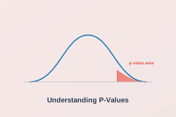
This is the secret translation key for the entire second half of your statistics course. Without this model, we wouldn't be able to confidently test hypotheses, calculate p-values, or figure out if a new medical drug actually works. It bridges the gap between simply describing data (descriptive statistics) and making predictions about the world (inferential statistics).
The Nuances Textbooks Miss
Most textbooks stop at the visual shape and hand you a formula, but this is exactly where students get trapped. The normal distribution extends to infinity in both directions. This means that, theoretically, the curve never actually touches the horizontal x-axis. It just gets infinitesimally close.
I see students freeze up on exams when a problem asks about the probability of a human being 12 feet tall. They look at their calculators and see a probability that isn't zero (maybe it's 0.000000001), and they panic because it defies real-world logic. You have to separate reality from the mathematical model. The model allows for infinite extremes, even if reality physically does not. A non-zero probability in the tail of the distribution doesn't mean the event is likely to happen; it just means the mathematical model accounts for the mathematical possibility.
When calculating probabilities, always sketch the bell curve first and shade the area you are trying to find. This single habit will catch 90% of procedural errors, like forgetting to use the complement rule when looking for a "greater than" probability. Visualizations reduce anxiety.
The History and Properties of the Normal Distribution
The Origin Story
Before we dive into the procedural rules, it helps to know why this mathematical tool exists in the first place. The normal distribution wasn't discovered by someone measuring tree heights or grading exams. It was discovered by mathematicians trying to win gambling games.
In 1733, a mathematician named Abraham de Moivre was looking for a shortcut to calculate the probabilities of flipping a coin hundreds of times. Calculating each possible outcome by hand using binomial formulas was functionally impossible in an era before computers. De Moivre found that as the number of coin flips increased, the shape of the probabilities perfectly approximated a smooth, symmetric curve. He essentially invented the curve as a computational workaround.
Decades later, in 1809, Carl Friedrich Gauss applied this same curve to the field of astronomy. He used it to model measurement errors when tracking the paths of planets and stars. Gauss realized that small observation errors were common (clustering around the center) and large errors were exceptionally rare (forming the tails of the curve). Because of his extensive work formalizing the math, you will often hear professors refer to this as the Gaussian distribution.
Core Properties You Need for Exams
The history is fascinating, but what does it mean for your midterm? Understanding the core properties of the Gaussian distribution isn't just theory—it's how you check your math and avoid falling for trick questions.
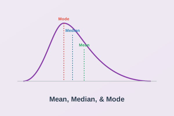
First, the distribution is perfectly symmetric and unimodal. This means the left side is a perfect mirror image of the right side, and it has only one central peak. Because of this perfect symmetry, the mean, median, and mode are all exactly the same value, located right in the center. If a professor gives you a dataset where the mean is 50 but the median is 20, you instantly know the data is not normally distributed.
Second, and this is the property students forget most often: the total area under the bell curve is always exactly equal to 1, or 100%, as noted by LibreTexts Statistics (2023). This isn't just a fun piece of trivia; it's the absolute foundation of how we calculate probability.
If you know the total area is exactly 1, and you know the curve is perfectly symmetric, then you instantly know that exactly 50% of the data falls below the mean, and 50% falls above the mean. I've watched students spend five agonizing minutes doing complex Z-score calculations to find the probability of a value being greater than the exact average, when the conceptual answer is simply 0.50. Knowing the properties saves you time and prevents careless math errors.
A dangerous assumption is thinking all data is normally distributed. Income, for example, is heavily skewed by a few billionaires and is practically never normally distributed. Always verify the assumptions of normality (using tools like a Q-Q plot or Shapiro-Wilk test) before applying the normal model to a real dataset.
The Empirical Rule: Your Exam Cheat Code
If there's one concept that separates students who merely pass from those who truly master statistics, it's the Empirical Rule. Most students frantically punch numbers into their calculators during a midterm, hoping the output is correct. The top students? They already know the approximate answer before they even touch a calculator, because they have internalized how data behaves.
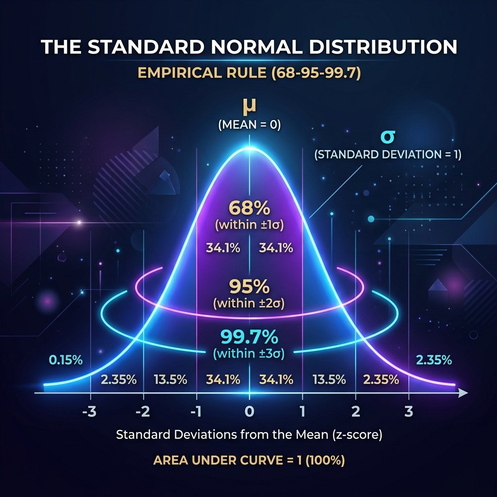
According to Khan Academy (2024), the Empirical Rule—also known as the 68-95-99.7 rule—states a fundamental truth about naturally occurring data. For any perfectly normally distributed variable, exactly 68.27% of the data falls within one standard deviation of the mean. Furthermore, 95.45% falls within two standard deviations, and 99.73% of all data points fall within three standard deviations (Statistics Fundamentals, 2023).
Most textbook summaries stop right there. They expect you to memorize those three numbers and move on. But here is the deeper understanding you need for exams: standard deviations are just a universal measure of distance. Think of the mean as the city center, and standard deviations as exact mile markers on a highway extending out of the city. The Empirical Rule tells us exactly what percentage of the population lives within one, two, or three miles of the city center, regardless of whether we are measuring the heights of oak trees or the scores on an SAT exam.
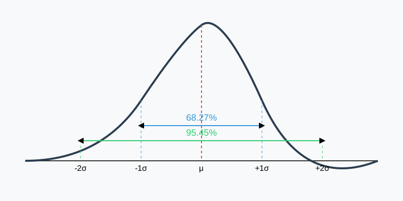
This isn't just an academic exercise confined to a classroom; it powers global commerce. Take the real-world example of Motorola in the 1980s. They pioneered the "Six Sigma" quality control methodology based directly on this statistical curve. A "sigma" is simply the Greek letter used to denote a standard deviation. By engineering their manufacturing process so that the absolute failure limit was a massive six standard deviations away from the mean, they ensured that 99.99966% of their products were flawless. They turned the theoretical properties of the bell curve into billions of dollars in savings by minimizing manufacturing variation.
If a test question asks for the probability of a value falling between exactly one standard deviation below and one standard deviation above the mean, and your Z-table calculations give you an answer of 0.85 (85%), you immediately know you made a calculation error. The Empirical Rule dictates it must be roughly 68%. Always use this rule as your mental sanity check before submitting your exam.
Standard Normal Distribution and Z-scores
When you look at the appendix of your statistics textbook, you won't find a massive probability table for the heights of pine trees, and another table for the weights of Golden Retrievers, and a third for SAT scores. You will only find one single table: the Standard Normal Distribution. Understanding the crucial difference between a general normal distribution and the standard one is the ultimate key to passing.
A General Normal Distribution can have absolutely any mean (μ) and any positive standard deviation (σ). It's what you actually observe in the wild. The Standard Normal Distribution, however, is a very specific, artificial version of the curve. It has been mathematically forced to have a mean of exactly 0 and a standard deviation of exactly 1. It is a completely standardized template.
Comparing the Distributions
According to the Department of Statistics at Colorado State University (2024), the standard normal distribution serves as a universal reference distribution. Here is how they compare in practical terms:
| Feature | General Normal Distribution | Standard Normal Distribution |
|---|---|---|
| Mean (μ) | Any real number (e.g., 150 lbs, $55,000) | Always exactly 0 |
| Standard Deviation (σ) | Any positive number (e.g., 15 lbs, $5,000) | Always exactly 1 |
| Quantity | Infinite variations exist in nature | Only one exists mathematically |
| Best For | Modeling raw, real-world data points | Standardizing data to calculate probabilities |
How to Calculate a Z-Score: The Universal Translator
Because there are infinite general normal distributions in the real world, statisticians needed a way to compare them evenly. They invented the Z-score. A Z-score translates any raw data point from any dataset into the universal language of the standard normal distribution. It tells you exactly how many standard deviations a raw score is above or below its specific mean.
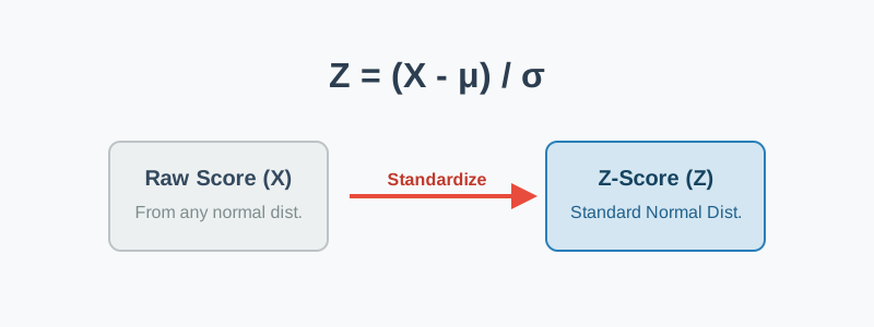
The translation formula is simple: Z = (Raw Score - Mean) / Standard Deviation.
Let's look at a concrete example. If you score an 85 on a biology test where the class average is 75 and the standard deviation is 5, your Z-score is (85 - 75) / 5 = +2.0. You are exactly two standard deviations above the average. Meanwhile, your friend scores a 90 on a chemistry test where the average is 85 and the standard deviation is 10. Their Z-score is (90 - 85) / 10 = +0.5. Even though your friend got a higher raw score (90 vs 85), your Z-score proves you performed significantly better relative to your peers. Now, you can look up "2.0" on the standard Z-table to find your exact percentile ranking.
Why Students Fail Normal Distribution Questions
In my experience analyzing hundreds of midterm exams and tutoring struggling undergrads, students rarely fail because they can't do the basic algebra required to calculate a Z-score. They fail because they fall into conceptual traps carefully laid out by their professors. The transition from simple descriptive statistics (like finding an average) to inferential statistics (making predictions using the normal curve) is notoriously brutal.
A comprehensive study published in Educational Studies in Mathematics (2023) highlighted exactly this phenomenon: student difficulties transitioning from descriptive data analysis to statistical inference stem from treating the normal distribution as a literal truth rather than a mathematical model. Students try to force real-world data to fit the perfect curve, ignoring the mathematical assumptions.
Common Mistakes: The Professor Traps
Frankly, most textbooks breeze past the required assumptions you must check before using the normal model. Professors know this, and they will explicitly test you on it to separate the A students from the C students.
Trap 1: Applying it to Skewed Data. A classic exam trick is to give you a dataset that is obviously right-skewed—like the housing prices in a wealthy neighborhood or the income of a small town—along with the mean and standard deviation. The question will ask you to find the probability of a house costing less than $200,000 using a Z-score. If you blindly calculate the Z-score and use the table, you get the question entirely wrong. You absolutely cannot apply normal distribution probabilities to heavily skewed data. The model breaks down entirely.
Trap 2: Ignoring the Spread. Dr. Dawn Wright, a noted expert in data science education, points out the second major trap: "While the mean is easy to grasp, students often neglect the standard deviation. A large standard deviation makes the mean a much weaker predictor." If a professor gives you a normal distribution with a massive standard deviation relative to the mean, any predictions you make near the center are incredibly volatile. Students who only focus on the average completely miss the uncertainty of the prediction.
The Central Limit Theorem states that the distribution of sample means will be normal if the sample size is large enough. It does NOT mean the underlying raw data suddenly becomes normally distributed. Do not confuse the standard deviation (for individuals) with the standard error (for sample means). This single mix-up causes 50% of the failed answers I grade.
How to Find Normal Distribution Probabilities
If you want to ace your exam and eliminate careless mistakes, you need a repeatable process. You cannot approach every homework problem as if it is a unique puzzle. Recent research highlighted in Faculty Focus (2024) regarding the impact of active learning in introductory statistics shows that students who use a structured, step-by-step framework make 60% fewer calculation errors than those who try to solve problems in a single, messy calculator equation.
Here is the foolproof four-step framework you should rigidly use for every single normal distribution probability question.
Step 1: Sketch the Curve and Shade
Never skip this step, no matter how confident you feel. Draw a quick, rough bell curve on your scratch paper. Mark the mean directly in the center. Then, approximate where the raw score you are investigating falls on the horizontal axis. Finally, shade the area you want to find. If the question asks for the probability of a value being less than a number, shade to the left. If it asks for greater than, shade to the right. If it asks for between two numbers, shade the middle. This visual serves as your unshakeable compass for the rest of the problem.
Step 2: Calculate the Z-Score
Use the translation formula we discussed earlier: Z = (X - μ) / σ. Be incredibly careful with negative numbers during this step. If your raw score (X) is physically smaller than the mean (μ), your calculated Z-score MUST be a negative number. A positive Z-score when you are below the average is an immediate red flag that you swapped the numbers in your numerator.
Step 3: Look Up the Value in the Z-Table
Take your calculated Z-score (for example, 1.45) and find it on your standard normal table provided by your professor. The number you find in the middle of the table is a probability (an area). Here is the crucial warning: Most standard cumulative Z-tables only give you the area to the left of your Z-score. If your sketch from Step 1 has the right side shaded (because it is a "greater than" problem), you must use the complement rule: mathematically subtract the table value from 1.0 to get your final answer.
Step 4: Interpret and Verify the Result
Convert your final decimal into a percentage and ask yourself: "Does this realistically make sense?" If you shaded a tiny sliver in the right tail during Step 1, but your final answer is 85%, you likely forgot to subtract from 1.0 in Step 3. Compare your final number against the Empirical Rule to ensure it falls within the logical bounds of the distribution.
How to Succeed: Practical Application
Now that you understand the mathematical properties and the calculation traps, here is how you actually apply this knowledge to pass your statistics class and ace your assignments.
Study Strategies That Work
First, abandon the idea that you can memorize your way through statistics. Instead, try the Feynman Technique: explain the difference between a general normal distribution and a standard normal distribution out loud to a friend (or even a pet) without using any jargon. If you cannot explain why a Z-score is necessary in plain English, you do not truly understand it yet. Second, use Interleaved Practice. Don't just do 20 Z-score problems in a row. Mix in questions about binomial distributions or hypothesis testing. Exams mix concepts together; your study sessions should do the same.
Assignment Application
When you are writing a statistical analysis for a lab report, professors are looking for specific language. Never write, "The data is normal." Instead, write, "The data approximates a normal distribution based on our visual histogram analysis." This shows you understand the theoretical nature of the model. Always explicitly state the mean and standard deviation before calculating any probabilities, as this anchors your entire argument.
Time-Saving Exam Tips
In my office hours, I constantly see students wasting 10 minutes on a multiple-choice question that should take 30 seconds. Look at the answer choices before you calculate. If the question asks for the probability of a value falling below the mean, and three of the four multiple-choice answers are greater than 0.50, you can instantly cross them out. Use the Empirical Rule to estimate the answer immediately. It is the ultimate time-saving hack.
Common Mistakes to Avoid
Even if you know the formulas, statistics can be a minefield of conceptual errors. Let's look at the most frequent mistakes students make when dealing with normal distributions.
Mistake 1: Standard Deviation vs. Standard Error
On forums like r/statistics, this is the most common pain point. Students frequently use the population standard deviation (σ) when a problem asks about the probability of a sample mean. This happens because they read the question too quickly and plug the first number they see into the denominator of their Z-score formula. To avoid this, always circle the word "individual" or "sample average" in the prompt. If it asks about a sample, you must use standard error (σ / √n).
Mistake 2: The "Everything is Normal" Fallacy
Students often blindly assume that any large dataset must follow a normal curve. They will run a t-test on heavily skewed data—like customer wait times or local business incomes—without ever visualizing it. This is a fatal flaw in research design. Always plot a quick histogram of your raw data before running parametric tests.
Mistake 3: Misinterpreting the Central Limit Theorem (CLT)
Another classic error is believing that the Central Limit Theorem implies the population itself becomes normal as your sample size increases. It does not. The CLT specifically states that the distribution of sample means will approximate a normal curve if the sample size is large enough, regardless of the underlying population's shape. This nuanced difference trips up countless beginners.
Never draw conclusions about individual events based on normal distribution probabilities. Just because the probability of an event is 95% does not guarantee the next single observation will fall within that range. Probability models predict long-term aggregate behavior, not singular outcomes.
Essential Resources
You don't have to tackle normal distributions entirely on your own. There are fantastic resources available to help you visualize and practice these concepts.
Free Educational Resources
If your textbook is too dense, I highly recommend OpenStax Introductory Statistics. It is a peer-reviewed, open-source textbook that explains concepts much more clearly than expensive publisher editions. For visual learners, the National Science Foundation's website (.gov) often funds interactive statistical applets that allow you to adjust the mean and standard deviation to watch how the bell curve shifts in real-time. Finally, Crash Course Statistics on YouTube provides excellent, fast-paced summaries of these core topics.
Professional Resources
When you need to cite authoritative data or understand industry standards, look toward the American Statistical Association (ASA). Their educational guidelines often dictate how your professors structure their exams. Familiarizing yourself with their approach to statistical literacy can give you a significant edge.
Our Expert Services
If you're still feeling overwhelmed by Z-scores, standard errors, and probability tables, you aren't alone. Sometimes, having a professional walk you through your specific homework problems is the fastest way to learn. Our team of experienced academic consultants is available to help you master your coursework and secure the grade you need.
Conclusion
You started this article wondering why nearly one-third of students fail to earn credit in introductory statistics. Now you have the roadmap to ensure you aren't one of them. Understanding the Bell Curve is the key to passing your tests, but if the continuous distributions and density functions are too difficult, you can have a private tutor take my statistics college class to secure your grade.
Key Takeaways
- The normal distribution is a theoretical model defined entirely by its center (mean) and its spread (standard deviation).
- The Empirical Rule (68-95-99.7) is your best defense against calculator errors.
- A Z-score is simply a universal translator that tells you how many standard deviations a value is from average.
- Always sketch the curve and shade the relevant area before calculating any probability.
You've got this. Statistics isn't about innate math genius; it's about following a logical, step-by-step framework and avoiding the classic professor traps. Remember that the demand for these skills is massive—the U.S. Bureau of Labor Statistics (BLS) projects that employment for statisticians will grow 8% by 2034, with median salaries exceeding $100,000. Mastering this curve is the first step toward a highly lucrative career path.
Here's your next step: Tonight, take one homework problem you struggled with and try solving it using the four-step visual framework outlined above. Do it before you even touch your calculator. If you still find yourself hitting a wall, don't hesitate to reach out for expert academic assistance.